Advanced musculoskeletal MRI at ultra-high field (7 T)

Siegfried Trattnig^1†, Klaus M Friedrich¹, Wolfgang Bogner¹ and Goetz H Welsch^1,2

¹ MR Center, High Field MR, Department of Radiology, Medical University of Vienna, Währinger Gürtel 18–20, A-1090 Vienna, Austria

² Department of Trauma Surgery, University Hospital of Erlangen, Krankenhausstr. 12, 91054 Erlangen, Germany

*Corresponding Author:

Siegfried Trattnig
MR Center, High Field MR, Department of Radiology
Medical University of Vienna, Währinger Gürtel 18–20
A-1090 Vienna, Austria
Tel: +43 140 400 6460
Fax:+43 140 400 6475
E-mail:siegfried.trattnig@ meduniwien.ac.at

Abstract

MRI at ultra-high field (7 T) offers high signal-to-noise ratio, which can be used beneficially in several different musculoskeletal applications. Spatial resolution in morphological imaging of small structures in joints such as cartilage, hip, wrist and foot can be significantly improved. The low sensitivity of multiparametric imaging for the visualization of cartilage ultra-structure can be enhanced and combined with high-resolution imaging. Sodium imaging suffering from low signal-to-noise ratio and low sensitivity benefits from the ultra-high field, thus sodium imaging that allows quantification of one important component of articular cartilage, proteogylcans (responsible for the biomechanical properties), is now attractive for clinical application. The better spectral resolution at 7 T makes 31phosphorus spectroscopy a promising tool for noninvasive evaluation of energy metabolism in healthy and diseased muscle.

Keywords

7 Tesla; ³¹phosphorus spectroscopy; articular cartilage ; multiparametric imaging; sodium imaging; ultra-high field; ultra-high resolution

Advanced morphological imaging at 7 T

Recently, high- (3 T) and ultra-high field (>3 T) whole-body MRI systems have played an increasingly important role in musculoskeletal imaging. However, to date, ultra-high field imaging systems are only used in research centers. In academic settings, 1.5 T scanners have been the gold standard for musculoskeletal MRI, but are now increasingly being replaced by 3 T systems.

The major advantage of MRI systems at 3 T and above is the increased capability to perform high-resolution morphological and especially biochemical imaging. At 1.5 T, most musculoskeletal tissues (e.g., cartilage, muscle, menisci, bone, tendon and ligaments) feature a low signal- to-noise ratio (SNR). Modern 3 T systems offer not only an increase in field strength, but also come along with advanced radiofrequency coil design, and new imaging sequences. Thus, the SNR is significantly increased, which can be translated into either higher temporal or spatial resolution for better morphological imaging.

The field strength-dependent SNR gain is outweighed by the frequency dependency of relaxation times, and the need to adjust sequence parameters (e.g., bandwidth and pulse parameters) to reduce artifacts, and not exceed the limits for the specific absorption rate (SAR). However, for 3 T systems, overall, problems have been sufficiently solved, but for ultra-high field systems, problems are even more severe, and have, to date, only been partly solved.

For example, more dedicated ultra-high field, multichannel, multielement coils need to be developed to allow the use of parallel imaging techniques, thus helping to overcome SAR restrictions. We also need to cope with increased inhomogeneity of the magnetic fields at ultra-high field systems.

Another limiting factor is the strength of the gradient systems used in the ultra-high field magnetic resonance (MR) scanners, which, to date, cannot be increased proportionally to B0; this limits the improvement of the inplane resolution at ultra-high fields compared with 3 T.

It should also be taken into account that, for many indications, it is not clear whether advanced image quality improves diagnostic accuracy. Ultra-high field MR images might further improve diagnostic confidence, but, based on our current experience, it is unlikely that diagnostic accuracy for these conditions, including morphologic imaging alone (without additional functional imaging), will be improved substantially with the transition from 3 to 7 T. For these and other common indications, where diagnostic accuracy is already high at 1.5 T, the relative advantage of 3 T or above might be to shorten acquisition time while maintaining an equivalent level of contrast and resolution, or to combine information from morphological and functional imaging.

However, there are indications in which accurate diagnosis was limited by the available SNR at 1.5 T, which now are likely to benefit from moving to 3 T scanners. In situations such as bilateral hip evaluations or peripheral nerve lesions, where large field-of-views as well as high spatial resolution are needed, 3 T, using high-resolution matrices combined with parallel imaging, might also be beneficial. Within the last several years, morphological imaging for various joints has advanced at different degrees. The following briefly summarizes some of the achievements, structured by anatomic regions.

Imaging the hip

MRI of the hip is challenging owing to the joint’s deep location in the body, which limits tissue penetration by surface coils, and thus, reduces SNR. The field strength-dependent SNR gain at 3 T compared with 1.5 T, and the resulting potential to use parallel imaging techniques, might be the keys to obtaining images with a large field-of-view and high spatial resolution in a reasonable scan time. It has been shown that high-resolution trabecular bone imaging of the proximal femur is feasible at 3 T, resulting in a voxel size of 0.234 × 0.234 × 1.5 mm³ and demonstrating superiority in the depiction of the bone structure compared with 1.5 T [1]. The diagnosis of femoral acetabular impingement, in particular, has become important over the last few years [2]. A study comparing hip imaging at 1.5 and 3 T demonstrated the capability of 3 T to improve the diagnosis of acetabular labral pathology owing to the higher spatial resolution, and also proposed that accurate hip imaging, without the need for a contrast agent, is feasible [3]. Owing to the complex anatomy of the hip joint, the use of isotropic 3D imaging sequences is becoming more and more accepted [4]. No data on in vivo imaging of the hip above 3 T have been published as yet.

Imaging the knee

Imaging at 1.5 T already provides very high image quality for knee imaging. Eckstein et al. evaluated the precision of assessment of cartilage volume, thickness and surface area of the femorotibial cartilage at 1.5 and 3 T, and found that results tend to be more reproducible at 3 T than at 1.5 T [5].

Chang et al. performed the first in vivo 7 T MRI study of the knee. They investigated the trabecular bone microarchitecture, and detected activity-related changes in Olympic fencers compared with healthy controls [6]. It has been shown that dual x-ray measurement of bone density, as currently used for the diagnostics of osteoporosis, is not sufficient to characterize bone quality, because, apart from the bone density, the trabecular bone achitecture contributes significantly to the mechanical strength, and thus, fracture risk [7,8]. Such bone structure is routinely characterized by microscopic CT [9,10]. However, it is not available for in vivo examination due to the high radiation dose. In vivo trabecular bone imaging is one of the emerging applications for high-resolution morphological MRI; this application, owing to the increased sensitivity to susceptibility and the resulting shortened T₂^*-relaxation times, truly benefits from moving to a higher field strength [11].

For cartilage imaging, up to a 2.4‑fold increase in SNR has been reported, when 3 and 7 T were compared using a fully-balanced, steady-state, free-precession pulse sequence (Figure 1). One study detected an increase in SNR from 3 to 7 T that was significant only for the gradientecho, but not for the fast spin-echo sequences [12]. Owing to limitations with the SAR, scan parameters for the fast spin-echo sequence had to be modified, which resulted in incomplete coverage of the knee joint, extensive artifacts and a less effective fat saturation. The contrast-to-noise ratio and image quality were increased for the gradient-echo and decreased for the fast spinecho sequences. When comparing 3 and 7 T, the level of confidence for diagnosing cartilage lesions was higher in the gradient-echo and lower in the fast spin-echo sequences; however, overall, the fast spin-echo sequences at 3 T had the highest confidence score. Evaluation of bone marrow edema was decreased at 7 T owing to the limited performance of the fast spin-echo sequences.

Kraff et al. performed a comparison between knee imaging at 1.5 and 7 T and also reported that, due to the SAR limitations with the fast spin-echo sequences, several measurements were needed for complete coverage of the knee joint [13]. They also confirmed that bone marrow edema was better visualized at 1.5 T than at 7 T. However, as yet, there is no study that verifies a statistically significant increase in diagnostic accuracy for the detection of common pathologies in the knee when moving to MR scanners with field strengths above 3 T.

Imaging the ankle

Bauer et al. performed trabecular bone imaging of the calcaneus; they concluded that 3 T results were more accurate than those calculated from the 1.5 T dataset [14]. Notably, the advances in visualizing trabecular bone structure were partially SNR independent. They assumed that the better performance at 3 T might have been due to increased sensitivity to susceptibility, enhancing the visualization of thin trabecular structures. The same group published data indicating that ankle abnormalities are better seen at 3 T than at 1.5 T; applying parallel imaging reduced the scan time by 56% [15].

Another group confirmed that image quality for imaging the ankle was significantly higher at 3 T than at 1.5 T [16]. In two of four readers, the sensitivity in detecting cartilaginous pathology at the ankle joint was enhanced significantly by imaging at 3 T compared with 1.5 T, using a fast spin-echo sequence. Differences between 1.5 and 3 T when balanced steady-state free precession and the spoiled gradient recalled sequences were used were insignificant, based on ratings by all the radiologists in that study. The sensitivities for detecting tendon pathologies were significantly higher at 3 T as opposed to 1.5 T for two of the radiologists in the same study. Specificities were similar for all readers at 1.5 and 3.0 T.

Imaging the ankle at 7 T is mainly limited by the lack of commercially available dedicated ankle coils. Thus, one group used an eight-channel head array coil for performing trabecular bone imaging at 7 T, and found that the relative noise enhancement factor was lower at 7 T than at 3 T for parallel imaging acceleration factors higher than three [17,18].

Imaging the shoulder

Any potential improvement in the accuracy of 3 T imaging of the shoulder is likely to be slight, given the already high degree of sensitivity and specificity at 1.5 T. The published literature currently comprises no direct comparison studies that evaluate the benefits of moving from 1.5 T to MR systems with higher field strengths for shoulder imaging. However, there are some studies that have evaluated shoulder imaging at 3 T. One of those studies demonstrated no statistically significant difference in the sensitivity and specificity of direct and indirect MR arthrography of the shoulder at 3 T with regard to the evaluation of rotator cuff, labral and long head of the biceps tendon tears [19]. Another study stated that direct MR arthrography shows a statistically significant increased sensitivity for the detection of partial-thickness articular surface supraspinatus tears, anterior labral tears and superior labrum anterior to posterior tears compared with conventional MRI at 3 T [20]. We assume that 3 T would not replace the need for MR arthrography completely, but may decrease the number of ambiguous cases that require additional arthrographic assessment. Probably owing to the lack of an appropriate coil, there are no reports on MRI of the shoulder at 7 T in the literature.

Imaging the wrist

The wrist is an especially challenging region because of the small size of the relevant anatomic structures, such as the intrinsic and extrinsic ligaments, the articular cartilage and the triangular fibrocartilage complex. Sensitivity, specificity and accuracy for imaging the triangular fibrocartilage complex pathology are higher at 3 T compared with 1.5 T [21].

Farooki et al. were the first to image the wrist above 3 T; they qualitatively compared 1.5 T with 8 T and concluded that 8 T was superior for the visualization of the infrastructure of the median nerve and in the definition of the boundaries of the carpal tunnel [22]. Other authors went on to quantify the difference between 1.5 and 7 T MRI of the wrist and found that SNR was approximately five-times higher in the tendon, bone, muscle and nerve [23]. These authors achieved a maximum spatial resolution of 0.16 × 0.16 × 1.50 mm³.

The New York University (NY, USA) research group uses an in-house-built radiofrequency eight-channel receive and four-channel transmit coil for wrist imaging, which provides the possibility to perform parallel imaging; the maximum spatial resolution they achieved was 0.08 × 0.08 × 2.00 mm³ [24].

In summary, morphologic MRI at 3 T has already been proven to be superior to 1.5 T in many musculoskeletal imaging applications and is widely used in the clinical routine; nevertheless, imaging at 3 T continues to improve. At 7 T, initial studies have demonstrated the great potential of those systems for ultra-high-resolution imaging, but several technical challenges remain to be solved. In the future, we might be able to entirely deploy the benefits of high- and ultra-high field imaging by combining ultrahigh- resolution morphological imaging with functional imaging techniques, even in the small joints of the human body.

Advanced functional (biochemical) imaging of articular cartilage

Proteoglycan-specific techniques Sodium imaging

Articular cartilage consists mainly of an extracellular matrix made of type II collagen, proteoglycan, chondrocytes and water [25]. Proteoglycan is made of a linear protein core to which many glycoproteins, known as glycosaminoglycans (GAGs) [26], are attached. Proteoglycan serves to crosslink the collagen fibrils in the extracellular matrix to provide both compressive and tensile strength to the matrix. In addition, the proteoglycan links restrict fluid flow through the matrix and thereby increase resistance to structural deformation.

The sulfate and carboxyl groups of the GAGs impart a negative fixed charge density (FCD) to the matrix. These negative ions attract positive counter ions (sodium) and water molecules and provide a strong electrostatic repulsive force between the proteoglycans. These osmotic and electrostatic forces are responsible for the swelling pressure of cartilage. The configuration of the proteoglycan macromolecules also contributes to the resistance of the matrix to the passage of water molecules and, hence, affects the mechanics of the cartilage in this fashion.

The onset of osteoarthritis (OA) is well understood to be associated primarily with biochemical phenomena. The ability to quantify these molecular changes will provide a tool for the early diagnosis of OA and treatment monitoring. The loss of proteoglycan from the extracellular matrix has been hypothesized to be the event that initiates the onset of OA [27,28].

The loss of proteoglycan with the onset of OA results in a reduction of FCD in cartilage. Maroudas et al. have shown that the FCD of cartilage is correlated to the GAG content of cartilage [29]. Since the FCD is counter-balanced by the sodium ions, loss of proteoglycan (hence GAG and FCD) due to cartilage degeneration results in the loss of sodium ions from the tissue. The loss of the negatively charged proteoglycan lowers the FCD in the tissue, thereby releasing positively charged sodium ions. A method has been proposed to quantify FCD both in vitro and in vivo by using sodium MRI and the Donnan equilibrium equation:

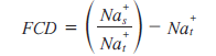
where Na_s is the sodium concentration in the surrounding synovial fluid and Na_t is the sodium concentration in the tissue [30].

Sodium MRI has been validated as a quantitative method of computing FCD and, hence, proteoglycan content in healthy humans [31–33]. Simultaneously imaging phantoms consisting of known concentrations of sodium enables the creation of a sodium concentration map of the cartilage. The corresponding FCD map can be calculated on the basis of the sodium map findings by using the above equation.

Healthy human cartilage FCD ranges from a concentration of 50 to 250 mM, depending on the age and location in the tissue [30]. As demonstrated in controlled cartilage degradation experiments [31,34], the sensitivity of sodium MRI is adequate for detecting small changes in proteoglycan content to the order of 5%.

Sodium MRI experiments were performed on the knee cartilage of healthy as well as earlystage OA patients at 4 T and demonstrated the feasibility of sodium MRI in computing proteoglycan loss in early-stage OA. The sodium 3D image data set was acquired with a voxel size of 5.3 μl (e.g., 1.1 × 2.0 × 2.4 mm) with an SNR of 12:1 in approximately 20 min [32].

By contrast, it took 30 min to obtain a 3D data set using a volume coil with the same SNR but an increased voxel size of 14.6 μl (e.g., 1.5 × 2.0 × 4.8 mm). With the effects of B1 inhomogeneity and voxel size accounted for, the surface coil provides an improvement in SNR by a factor of 2. Alternatively, an image can be obtained with a surface coil in 25% of the time that it takes to acquire one with a volume coil image with an identical SNR and voxel size. Results from this study revealed that cartilage of healthy subjects had a mean FCD with a concentration of 182.9 mM in healthy as well as osteoarthritic patients. Furthermore, its utility in measuring FCD changes in an animal model of OA has been described [35].

The major advantage of sodium MRI, especially of cartilage, is that it is highly specific to proteoglycan content and, since the sodium from surrounding structures in the joint is low (<50 mM), cartilage can be visualized with very high contrast without the requirement for any exogenous contrast agent such as that in delayed gadolinium enhanced MRI of cartilage (dGEMRIC) [36]. It can be used to quantify early molecular changes in OA.

The disadvantages of sodium MRI are that it requires field strengths greater than 3 T to obtain quality sodium images that enable accurate quantification of cartilage FCD. Furthermore, owing to the limitations of gradient strengths and other hardware requirements, most of the sodium imaging experiments reviewed here employed echo times (TE) of under 2 ms. Since the fast T₂ decay of cartilage lies in the range of 1 to 2 ms, substantial signal is lost before the acquisition. This is a major contributor to the low SNR of sodium compared with conventional proton MRI. Additionally, the sodium gyromagnetic ratio (g) is a quarter that of protons, hence sodium MRI requires four-times stronger gradients to obtain images with identical resolution to that of proton MRI. Nevertheless, the resolution is not only a function of the gyromagnetic ratio, but also of the receiver bandwidth. The MR sensitivity for 23Na is only 9.2% of the ¹H MR sensitivity, and the in vivo concentration is approximately 360-times lower than the in vivo water proton concentration. The combination of these factors results in a 23Na signal that is approximately 4000-times smaller than the ¹H signal.

However, recent advances in magnet technology, improved gradient performance and multicoil RF technology (parallel receive as well as transmit) may enable one to achieve ultra-short TE (<200 ms) that can significantly improve resolution and SNR. Radiofrequency coil technology (multiple channel capability) and parallel imaging approaches and tuned preamplifiers would further contribute to high SNR. These advances may potentially make clinical sodium MRI feasible on 3 T scanners. Furthermore, the recent proliferation of 7 T whole-body MRI scanners in clinical research centers could have a significant impact on sodium MRI and its potential for clinical use. Since SNR scales as B7/2 [37–39] and the lack of B1 penetration and B0 susceptibility are issues that pose problems with proton imaging, sodium MRI can be particularly advantageous at higher fields. Furthermore, unlike proton T₁, which increases with field, as the T₁ of sodium is predominantly due to quadrupolar interaction, it may not change appreciably at higher field. This retains the rapid averaging capability of sodium MRI even at high fields. The low g of sodium will also mean significantly lower power deposition compared with proton imaging. It is therefore very likely that, with the improved SNR, sodium MRI at 7 T and higher fields would emerge as a robust tool for quantitative imaging of cartilage. Although sodium MRI has high specificity and does not require any exogenous contrast agent, it does require special hardware capabilities (multinuclear), specialized RF coils (transmit/receive) and likely 3D ultra-short TE sequences. These challenges currently limit the clinical use of sodium MRI at standard clinical scanners. Nevertheless, this technique has been successfully demonstrated in vivo on pigs, in human wrists and in a human knee [33,40,41].

We have recently applied sodium imaging in patients after matrix-associated autologous chondrocyte transplantation (MACT). Our sodium measurements were performed using a 23Na-only (78.61 MHz) circularly polarized transmit/ receive knee coil with the inner diameter of 19 cm (Stark Contrast, Erlangen, Germany). A reference sample containing 308 mM of NaCl was fixed to the inner surface of the sodium coil to normalize the inter-scan signal variability. With the application of a 7 T whole-body system and modified 3D gradient recalled echo (GRE) sequence we achieved a significantly higher SNR and spatial resolution compared with customary used GRE sequences. This allowed us to visualize even the femoral condyle cartilage layer, which is thinner than the patellar cartilage, but is the preferred location for cartilage transplantation. The reports on sodium imaging of the knee joint have so far focused on the patellar cartilage layer. The resolution we achieved was even high enough to visualize the thin cartilage layer of the adjacent proximal tibio–fibular joint (Figure 2). In our patient group sodium imaging allowed differentiation between different concentrations of sodium and, hence, GAG in different portions within the transplants, which underscores its strength in the overall evaluation of cartilage transplants in contrast to the limited biopsy sample evaluation. The sensitivity of sodium imaging was high enough to detect sodium and, hence, GAG concentrations in one transplant, which was even higher compared with normal hyaline cartilage adjacent to it. A similar finding in dGEMRIC revealed higher postcontrast T₁ values compared with normal cartilage, a finding that seemed to be paradoxical and raised the suspicion of an error in the dGEMRIC measurement.

We found a good correlation between sodium imaging and dGEMRIC in the quantification of the GAG concentration in patients after MACT.

In summary, sodium imaging at 7 T becomes clinically useful and will establish a new standard in biochemical imaging of articular cartilage with its direct correlation to GAG concentration, the component of the ultrastructure of cartilage that is lost in the earliest stages of OA and plays the most important role in the biomechanical properties of cartilage.

dGEMRIC at 7 T

For the visualization of GAGs, besides sodium imaging, dGEMRIC [42,43] has gained significant importance. The dGEMRIC is based on the fact that proteoglycans contain negatively charged side chains that lead to an inverse proportionality in distribution of the negatively charged contrast agent molecules with the concentration of proteoglycans. Consequently, T₁, which is determined by the Gd‑DTPA2- concentration, becomes a specific measure of tissue proteoglycan concentration. The value of this technique and the possible clinical applications have been repeatedly reported [44–46].

In the majority of these studies only T₁ after penetration of Gd‑DTPA^2- (T₁[Gd]), has been used. However, from studies on cartilage implants and from studies on higher field strength (3 T), it has been reported that the d‑relaxation rate R1 calculated as 1/T₁(Gd) minus 1/T₁ precontrast, should be more representative of Gd‑DTPA^2- concentration, where T₁ precontrast = T₁ before contrast administration [47,48].

Recently, whole-body scanners operating at 7 T were installed and are increasingly used for clinical studies on patients [49–51]. So far, no studies are known that describe the contrast agent behavior at this field strength. From earlier studies it is known that the relaxivity of contrast agents decreases with increasing field strength [52], which may significantly influence the efficacy of dGEMRIC technique. The ultra-high magnetic field at 7 T with the higher SNR ratio offers high-resolution protocols in articular cartilage that have not been possible so far in vivo. Recently a 3 T application of a dual-flip angle excitation pulse GRE technique was demonstrated to be comparable to standard inversion recovery (IR) sequence in the evaluation of cartilage implants but provided a significant reduction in scan time [53].

The aim of our study was therefore twofold:

• To compare standard T₁ mapping IR sequence with a dual flip angle excitation pulse GRE technique in phantom at 3 and 7 T as well as in volunteers at 7 T;

• To evaluate the feasibility of the dGEMRIC technique at 7 T in volunteers, in particular to define how large the range is between preand postcontrast T₁ values at 7 T, which is a prerequirement for the application of the dGEMRIC technique in patients.

On phantom studies the comparison of IR and dual-flip angle 3D GRE showed a lower correlation in the longer range of T₁ values from 800 ms and higher. Additionally, only half of the central slices demonstrated a significant correlation between IR and GRE. The mean calculated T₁ precontrast and T₁(Gd) values from the anterior, central and posterior femoral condyle of the volunteers are shown for IR (Figure 3A) and dual-flip angle excitation pulse GRE sequence (Figure 3B). The T₁ values pre- and postcontrast differed significantly between IR and GRE techniques, however, the difference between T₁ values pre- and postcontrast was lower with GRE T₁ mapping technique, since the postcontrast drop of T₁ values was more pronounced with IR compared with GRE technique. This may pose a problem in clinical application of the dGEMRIC technique based on GRE at 7 T. Figure 4 shows an example of pre- and postcontrast T₁ maps calculated from IR dGEMRIC measurements. On both images cartilage is pseudo-colored to better delineate its T₁ values.

Similar separation between 1/T₁ (R1) precontrast) and 1/T₁ (R1) (Gd) was observed at the ultra-high field of 7 T, compared with reported values at 3 T, although a lower contrast agent relaxivity was expected at 7 T, which could lead to less separation [46]. The effect on behaviour of contrast agents at different field strengths depends on two basic mechanisms: the nuclear magnetic relaxation dispersion and the fielddependent relaxation of tissue [54]. The nuclear magnetic relaxation dispersion or relaxivity of a paramagnetic ion to water protons, described by the Solomon-Bloembergen–Morgan equation, is higher at lower magnetic field strengths and decreases at higher magnetic fields [55]. A recent report described that at a field strength of 3 T the use of T₁(Gd) as a measure of Gd‑DTPA^2- distribution may be less suitable at 3 than 1.5 T but may still be useful if precontrast T₁ values are also calculated [48]. From the calculated T₁ values of IR sequence at 7 T, this statement can be used for 7 T as well, and the use of T₁(Gd) seems to be similarly appropriate at 7 T as an index of Gd‑DTPA^2- concentration in cartilage than at 3 T.

The dual-flip angle excitation pulse GRE technique provided unreliable results at 7 T, which may be due to several reasons: first, the optimal flip angle for the GRE method is tissue T₁ dependent, which means that for 7 T different sets of flip angles compared with 3 T for the preand postcontrast T₁ measurement should be used. Second, gradient-echo sequences are more prone to static magnetic field inhomogeneities. With the reduced wavelength of RF waves in the human body, the inhomogeneous power absorption and formation of so-called ‘hot spots’ are of increased concern, particularly at 7 T and have to be considered in IR sequences. This is mainly caused by the dielectric properties of tissues [56–58].

In conclusion, this study shows for the first time that dGEMRIC is feasible at 7 T. The difference between pre- and postcontrast T₁ values is high enough to be useful for quantification with the dGEMRIC technique and the combination of 7 T ultra-high resolution together with functional MR seems to be possible and may be an important step into molecular imaging of articular cartilage in the near future.

Collagen-fiber- & water-specific techniques

To visualize the ultrastructure of articular cartilage, the intervertebral disc and other soft tissues in the musculoskeletal system, a variety of different methodologies are available. Depending on the anatomic localization and following the available coil configurations, within the different large and small joints as well as within the whole spine, biochemical MRI can be achieved to assess the constitution of the specific tissues. T₂-relaxation time mapping is the most widely used technique and was first used to describe the composition of hyaline articular cartilage in the knee joint based on its collagen structure and hydration.

Besides the knee joint, the cartilage of the hip joint and initially of the ankle, the shoulder, the elbow and the wrist are also goals of biochemical T₂ MR studies. As large patient groups suffer from OA of different joints and, thus, degenerative cartilage disease, to describe articular cartilage at high and ultra-high fields is becoming increasingly important. Besides idiopathic OA, reasons for the development of OA are cartilage defects in younger patients due to different reasons, which when untreated lead to OA. Hence, surgical and nonsurgical treatment options need sophisticated follow-up to show their potential benefit in the prevention of degenerative cartilage disease. Basically, articular cartilage is complex, dense, connective tissue that relies on the diffusion of solutes for its nutrition [59]. The extracellular matrix is responsible for the biomechanical properties of articular cartilage, mainly composed of water (~75%), collagen (~20%) and proteoglycan aggregates (~5%) [59,60]. Water either freely moves throughout the matrix or is bound to macromolecules. Collagen in hyaline cartilage is largely type II, which creates a stable network throughout the cartilage. The negatively charged proteoglycans are composed of a central core protein to which GAGs are bound. Articular cartilage is stratified primarily according to the orientation of collagen within a 3D network [60,61].

Although the differentiation of which components of articular cartilage are visualized by the specific sequence is not completely possible, the classic biochemical MR methodology that focuses on the collagen content of articular cartilage is T₂ mapping [62]. In addition to the transverse relaxation time (T₂) of articular cartilage, recently, T₂^* relaxation has been discussed for the depiction of the collagen matrix [63]. For both methodologies, according to the stratification of cartilage from the subchondral bone to the cartilage surface, zonal evaluation of articular cartilage is crucial.

Within the knee joint, besides biochemical T₂ mapping of articular cartilage lesions and the monitoring of osteoarthritic changes of the cartilage, the application of T₂-mapping methodologies in the meniscus has become more of a focus of recent research. Furthermore, meniscal lesions might also lead to OA. Normal human meniscal tissue has been found to be composed of approximately 70% water, 25% collagen and 1% GAGs with a regional variation due to the location in the knee joint. The predominantly dense framework is based on type I collagen fibers in a mainly circumferential orientation [64]. Within the meniscus T₂ mapping (with reduced TE) and T₂^* are initially used with promising results.

One other large group of patients in the musculoskeletal field, besides OA, are people suffering from back pain and especially from low back pain (LBP). Degenerative disc disease is regarded as the most prevalent cause of LBP, even though the pathophysiological correlations between pain and disc degeneration are not fully understood as the problem of LBP is multifactorial. In intervertebral discs (IVDs), the annulus fibrosus consists of fibro-cartilage and its function as a rigid containment for the nucleus pulposus (NP) accounts for its fibrous structure and low water content. The gelatinous structure of the NP, however, consists mostly of water, bearing a low yield of collagenous material. Degeneration of IVDs is initiated by the incapacity of disc cells to maintain a highly hydrated proteoglycan-rich matrix of the NP as well as a loss of the collagen structure that affects the mechanical integrity of the IVDs. The IVDs mechanical function in distributing axial loads and absorbing shock while providing flexibility relies heavily on the hydrodynamic capabilities of the NP. Owing to the high reliance of the IVDs on their biochemical composition, functional MR techniques are becoming increasingly important in the diagnosis and treatment followup of patients with LBP. T₂ and T₂^* mapping are able to visualize the IVDs. When analyzing the IVDs using T₂- or T₂^* -mapping techniques, the biochemical stratification of the IVDs, as an increase in T₂ or T₂^* values from annulus fibrosus to the NP, has to be taken into account. MRI is the method of choice to depict the morphological and biochemical status of IVDs, nevertheless, to date, this remains only possible at high fields, whereas at ultra-high fields very initial results are highly limited owing to the lack of body coils.

T₂-relaxation time mapping of articular cartilage at high & ultra-high fields

The T₂ of cartilage is a sensitive parameter for the evaluation of changes in water and collagen content and tissue anisotropy [62]. Cartilage T₂ reflects the interaction of water and the extracellular matrix on a molecular level. The collagen fiber orientation defines the layers of articular cartilage. Thus, the 3D organization and curvature of the collagen network, influenced by water mobility, the proteoglycan orientation and the resulting magic angle at 55° (with respect to the main magnetic field [B₀]; where the magic angle is a physical phenomenon influencing image characteristics) influence the appearance of T₂ [61,65]. In healthy articular cartilage, an increase in T₂ values from deep to superficial cartilage layers can be observed, based on the anisotropy of collagen fibers running perpendicular to cortical bone in the deep layer of cartilage [66]. Histologically validated animal studies have shown this zonal increase in T₂ values as a marker of hyaline or hyalinelike cartilage structure after cartilage repair procedures in the knee [67,68]. To visualize this zonal variation in vivo, high spatial resolution is essential, which can already be achieved at highfield MR, together with dedicated multichannel coils in clinical approaches. Nevertheless at ultra-high field MR, the possibilities of T₂ mapping may still increase and a higher spatial resolution might provide additional benefits in future approaches. Hence, for musculoskeletal MRI at ultra-high fields, the utilization of biochemical sequences and, for example, the use of T₂-mapping techniques will increase.

Analyses of T₂-relaxation times within the knee have previously been performed usually at 1.5 T or more recently at 3.0 T [69–71]. These studies have demonstrated its feasibility as well as the benefit of a functional evaluation of articular cartilage to see premorphologic abnormalities. Studies comparing T₂ relaxation at 1.5 and 3.0 T reported a less pronounced dependence on the magnetic field strength compared with longitudinal T₁ relaxation, however, a shortening of T₂ values at 3.0 T by approximately 10% and by 10–20% at 4.0 T compared with 1.5 T have been published [72–74]. However, T₂ values reported in literature depend, to a great extent, on the sequence evaluated. Stanisz et al. found their T₂ values at both 1.5 and 3.0 T [73] to be similar to those of Smith et al. [66], but higher compared with the evaluation of Gold et al. [72]. All three study groups, however, used different sequences in their quantitative evaluation of T₂ with a different length of the TE. Our group uses a traditional multi-echo spin-echo technique for standard T₂ mapping, showing slightly lower T₂-relaxation time values of articular cartilage of the knee at 7.0 T to studies using a similar T₂ technique at 3 T [71]. Although an available comparison of T₂-relaxation times at 3.0 and 7.0 T did not find a shortening of T₂ values [75], an ongoing study by our group is showing a slight, yet significant, decrease of T₂-relaxation times from 3.0 to 7.0 T. The different cartilage locations (patella, femur and tibia) were evaluated in one study by our group at 7.0 T using SE T₂ mapping [63] and showed comparable results to those of Pakin et al. with a significant decrease in T₂ values between femoral and tibial weight-bearing cartilage (Figure 5) [75]. Furthermore, the patella showed lower T₂ values than the femoral condyle. In a study by Mosher et al. the T₂ values of the femoral condyle, the tibia and the patella were assessed and showed roughly equivalent results at all three anatomic regions [76]. However, in a later study by the same group, observing T₂ relaxation after exercise, variable behavior of femoral and tibial cartilage was observed [70], possibly indicating different behavior of femoral and tibial cartilage. Hence, at high field and ultra-high fields, T₂-relaxation time mapping cannot be seen as a method preparing absolute T₂ values of a specific anatomic cartilage region. Furthermore, in the evaluation of OA, T₂-relaxation times are again providing different results [46].

In cartilage repair tissue, nevertheless, global (bulk; full-thickness) T₂ and in particular, zonal T₂ evaluations have shown very promising results. Hence, in the follow-up after MACT, the visualization of cartilage repair tissue maturation was possible at high fields and a differentiation between cartilage repair tissue at the patella and the medial femoral condyle could be achieved [71,77,78]. Comparable to the results at 3.0 T, also at 7.0 T multi-echo spin-echo T₂ mapping could be used in the assessment of patients after cartilage repair [63]. Furthermore, using T₂ mapping, cartilage repair tissues after different repair procedures could be distinguished at high fields [79], whereas cartilage repair tissue after microfracture – histologically seen as fibrocartilage – shows no zonal increase from deep to superficial cartilage aspects, and repair tissue after MACT – histologically reported as hyaline-like – shows a significant stratification.

As mentioned previously, in OA, T₂ mapping has shown varying results [46,69,80] and the role of T₂ as an absolute quantification parameter must be further analyzed. Thus, it is not yet clear whether a slight increase or decrease in T₂-relaxation times can be correlated to morphological changes. For the evaluation and the validation of T₂-relaxation time mapping in OA in particular, ultra-high field may in future provide a clearer insight into these early changes of the collagen matrix, although this cannot be proven at present.

T₂*-relaxation time mapping of articular cartilage at high & ultra-high fields

In addition to standard SE T₂-relaxation, T₂*‑weighted 3D gradient-echo articular cartilage imaging has shown reliable results in the evaluation of osteoarthritic cartilage changes of the knee [81]. In recent studies, T₂* mapping, with its short scan times, was correlated to standard SE T₂ showing information comparable to that obtained for articular cartilage using SE T₂, but with overall lower T₂* values (ms) [82,83]. Furthermore, for T₂*, a clear zonal variation between the deep and superficial cartilage layers was also described for healthy cartilage.

In cartilage repair, T₂* mapping provides promising results and whilst in patients after cartilage transplantation techniques, a zonal stratification was visible, in patients after microfracture this stratification could not be found [82]. Thus, for standard T₂, as well as for T₂*, zonal assessment of healthy and altered articular cartilage is crucial.

Nevertheless, for T₂*, the zonal variation between the subchondral border and the cartilage surface might have another explanation, owing to the influence of local susceptibility fields on T₂* and requires further study. These local fields can operate at a macroscopic level (i.e., at the bone/cartilage interface) or at the microscopic level (i.e., associated with the underlying microstructure of the cartilage). If these processes produce local changes in the macroscopic static field gradients, this might be more distinct in the deep cartilage zone. This problem in the evaluation of the cartilage near the subchondral bone plate might also account for the differences in the zonal stratification between T₂ and T₂*, with a clearer increase from the deep to superficial relaxation times in T₂* compared with T₂. Furthermore, T₂* has not been sufficiently validated for its use in cartilage, and it could be that T₂* visualizes different properties of articular cartilage in addition to collagen and including, perhaps, proteoglycan aggregates. In ultra-high fields, T₂* could be used in the depiction of healthy hyaline cartilage and in patients after MACT [63]. Furthermore, an ongoing study by our own group comparing the performance of T₂* at 3.0 and 7.0 T provides (comparably to standard SE T₂) lower T₂* values at 7.0 T (Figure 6). Again, however, histological validation has to prove the properties of articular cartilage depicted by T₂* at high and ultra-high fields.

Advanced metabolic imaging at 7 T

Musculoskeletal phosphorus MR spectroscopy:

Another MR method that has the potential to become increasingly important in future musculoskeletal high-field MR and might have a comeback is phosphorus MR spectroscopy (³¹P‑MRS). ³¹P‑MRS has become a popular tool among muscle physiologists in the last century, since it reveals the major factors of muscle metabolism noninvasively [84–87]. In particular, it allows the quantification of high-energy phosphates and intracellular pH [85], which are important indicators for muscular metabolism, especially in short-term bioenergetics. Consequently, after the first successful human applications, ³¹P‑MRS was expected to enter clinical routine rather fast. Nowadays, several groups use this method regularly for the investigation of muscle diseases [88–91], but its application for clinical routine is not widespread [84,92]. On the contrary, ³¹P‑MRS remained to some extent a research tool for physiology and pathology. On clinical scanners this can be explained by the following reasons: special hardware requirements are usually not met; the spatial resolution of ³¹P‑MRS is not as good as for 1H‑MRI/MRS; and ³¹P‑MRS experiments may be very time consuming.

Conversely, almost all MR applications should benefit from an increase in field strength, owing to increasing SNR and MRS in particular, by an increase in spectral resolution. Practically, several 1H‑MRI/MRS methods are facing severe limitations at 7 T, while ³¹P‑MRS does not have these limitations. Rather, there are several physical properties of ³¹P nuclei that dramatically alleviate the use of ³¹P‑MRS at a higher field strength. Owing to a much lower Larmor frequency, SAR limits are usually not met at 7 T. The large spectral frequency dispersion allows easy automatic data processing. Water/fat suppression at higher fields becomes increasingly unreliable, but no such suppression is necessary in ³¹P‑MRS. Increasing T₁-relaxation times of metabolites observed in 1H‑MRS [93] are reducing the net increase in SNR per unit time, unlike in ³¹P‑MRS, where the T₁ of most metabolites is decreasing. This leads to either additional SNR per unit time or reduced measurement times. Finally, the spectral resolution was shown to improve significantly from 3 to 7 T [94]. For comparison, two example spectra are displayed in (Figure 7A & B) to illustrate the improved spectral quality of ³¹P‑MRS spectra in the human calf muscle at 7 T compared with 3 T.

Well-known metabolites that can be quantified by ³¹P‑MRS include the high energy phosphates phosphocreatine (PCr), ATP, ADP and inorganic phosphate (Pi) which are all involved in the creatine kinase reaction. One of the most important features of ³¹P‑MRS is its ability to monitor time-dependent changes of metabolite concentrations. In so-called ‘dynamic’ MRS studies, the muscle can be easily stressed with exercise inside the magnet bore while the biochemical response can be monitored with a time resolution of a few seconds [87]. At the same time the spectral distance between Pi and PCr allows an accurate determination of the intracellular pH. Owing to the decrease in T₁ this time resolution can even be improved at 7 T compared with lower field strengths.

Different indices such as the rate of PCr decrease, the drop of pH, the initial rate of PCr recovery and the recovery of ADP were used to characterize muscle energetics in vivo. The initial PCr recovery is correlated with the maximum oxidative rate in tissue, while the recovery of ADP is considered the most sensitive and reliable noninvasive measure of mitochondrial dysfunction [95]. Recently, its ability to identify malfunctions in energy metabolism was demonstrated in a patient with myasthenia gravis [88].

A large clinical spectrum of mitochondrial disorders [96–98] and glycolytic defects [99] can be studied with ³¹P‑MRS. ³¹P‑MRS is the most sensitive and specific method for assessment of skeletal muscle mitochondrial rate of ATP production, especially during recovery [96]. Prolonged rate of PCr recovery, faster pH recovery and a delay in ADP recovery can be observed in mitochondrial dysfunctions.

³¹P‑magnetic resonance spectroscopy is also a suitable tool for physiopathologic studies. It has become an interesting tool in the study of systemic diseases such as renal or heart failure, and peripheral vascular or thyroid disease that is affecting muscle metabolism [92]. It also allows the investigation of gene function on metabolism [100] and can be an excellent tool for therapeutic trials [89,101], since unlike muscle biopsy, it can be easily applied repeatedly to assess treatment response over long periods [102].

Other ³¹P metabolites that are of interest, especially for oncology, include phosphocholine (PC) and phosphoethanolamine. The elevation of PC in ³¹P‑MRS and total choline in 1H‑MRS is one of the most widely established characteristics of cancer cells. Several studies have detected high levels of PC or phosphoethanolamine compared with normal tissues [103,104]. A glycerophosphocholine (GPC) to PC switch appeared to be an early phenotypic change during carcinogenesis as observed in benzo(a)pyrene immortalized cells where instead of GPC, PC became the major choline phospholipid metabolite. Since ³¹P‑MRS allows the separation of GPC and PC, it is in contrast to 1H‑MRS, a more specific method for the study of the metabolic characteristics of cancer.

At lower field strength, ³¹P‑MRS was rarely used in vivo for cancer research since good localization of relatively small volumes with sufficient SNR is required for the definition of the tumor region. Good localization is usually not critical in studies on muscle metabolism, where typically localization based on surface coils is sufficient. However, at 7 T, even localized ³¹P‑spectra can be acquired in clinically acceptable measurement times of 2 min (Figure 7C).

Thus, the opportunities of ³¹P‑MRS are manifold and range from the assessment of metabolic disorders for both diagnostic use and therapy monitoring to research in a variety of other diseases including diabetes research [86,90,105,106]. Recently, ³¹P‑MRS have become more widely available from commercial vendors even at lower fields. As soon as the additional value of multinuclear MRI/MRS techniques at ultra-high fields are recognized and more MR scanners are equipped with the necessary hardware, the long anticipated advance in ³¹P‑MRS can be realized.

Future perspective

The major advantage of high-field and ultrahigh- field MR is the shift from morphological to biochemical and metabolic imaging, techniques that normally suffer from low sensitivity at a standard field strength (1.5 T). The high SNR ratio provided by the higher field systems provides biochemical and metabolic imaging in reasonable scan times, which promotes its widespread clinical application. This development allows the diagnosis of diseases in their earliest stages such as OA, degenerative disc disease and muscle disease before morphological changes occur. Thus, the basic imaging requirements are available for the evaluation and follow-up of new disease-modifying drugs and the trend to a more personalized medicine.

Financial & competing interests disclosure

This work was supported by Austrian Science Funds FWFTRP‑Projekt L243-B15, FWF Projekt P18110-B15 and FWF-TRP 494-B05. Funding for this study was provided by the project “Vienna Advanced Clinical Imaging Center” (VIACLIC), within the “Vienna Spots Of Excellence” program; a collaboration of the Medical University of Vienna and Siemens Austria. The authors have no other relevant affiliations or financial involvement with any organization or entity with a financial interest in or financial conflict with the subject matter or materials discussed in the manuscript apart from those disclosed.

No writing assistance was utilized in the production of this manuscript.

Papers of special note have been highlighted as:
*of interest
* of considerable interest

References

1. Krug R, Banerjee S, Han ET, Newitt DC, Link TM, Majumdar S: Feasibility of in vivo structural analysis of high-resolution magnetic resonance images of the proximal femur. Osteoporos. Int. 16(11), 1307–1314 (2005).
2. Mamisch TC, Werlen S, Zilkens C et al.: Radiological diagnosis of femoroacetabular impingement. Radiologe 49(5), 425–433 (2009).
3. Sundberg TP, Toomayan GA, Major NM: Evaluation of the acetabular labrum at 3.0-T MR imaging compared with 1.5-T MR arthrography: preliminary experience. Radiology 238(2), 706–711 (2006).
4. Mamisch TC, Bittersohl B, Hughes T et al.: Magnetic resonance imaging of the hip at 3 Tesla: clinical value in femoroacetabular impingement of the hip and current concepts. Semin. Musculoskelet. Radiol. 12(3), 212–222 (2008).
5. Eckstein F, Charles HC, Buck RJ et al.: Accuracy and precision of quantitative assessment of cartilage morphology by magnetic resonance imaging at 3.0T. Arthritis Rheum. 52(10), 3132–3136 (2005).
6. Chang G, Regatte RR, Schweitzer ME: Olympic fencers: adaptations in cortical and trabecular bone determined by quantitative computed tomography. Osteoporos. Int. 20(5), 779–785 (2009).
7. Goldstein SA, Goulet RW, Mccubbrey D: Measurement and significance of 3-dimensional architecture to the mechanical integrity of trabecular bone. Calcif. Tissue Int. 53, S127–S133 (1993).
8. Kleerekoper M, Villanueva AR, Stanciu J, Rao DS, Parfitt AM: The role of 3-dimensional trabecular microstructure in the pathogenesis of vertebral compression fractures. Calcif. Tissue Int. 37(6), 594–597 (1985).
9. Borah B, Dufresne TE, Chmielewski PA, Gross GJ, Prenger MC, Phipps RJ: Risedronate preserves trabecular architecture and increases bone strength in vertebra of ovariectomized minipigs as measured by three-dimensional microcomputed tomography. J. Bone Miner. Res. 17(7), 1139–1147 (2002).
10. Ding M, Odgaard A, Linde F, Hvid I: Age-related variations in the microstructure of human tibial cancellous bone. J. Orthop. Res. 20(3), 615–621 (2002). n Bone remodeling mechanisms are studied to provide a thorough understanding of the microstructure of cancellous bone, crucial for diagnosis, prophylaxis and treatment of age-related skeletal diseases.
11. Krug R, Carballido-Gamio J, Banerjee S, Burghardt AJ, Link TM, Majumdar S: In vivo ultra-high-field magnetic resonance imaging of trabecular bone microarchitecture at 7 T. J. Magn. Reson. Imaging 27(4), 854–859 (2008).
12. Stahl R, Krug R, Kelley DAC et al.: Assessment of cartilage-dedicated sequences at ultra-high-field MRI: comparison of imaging performance and diagnostic confidence between 3.0 and 7.0 T with respect to osteoarthritis-induced changes at the knee joint. Skeletal Radiol. 38(8), 771–783 (2009).
13. Kraff O, Theysohn JM, Maderwald S et al.: MRI of the knee at 7.0 Tesla. Rofo: Fortschritte Auf Dem Gebiet Der Rontgenstrahlen Und Der Bildgebenden Verfahren 179(12), 1231–1235 (2007).
14. Bauer JS, Monetti R, Krug R et al.: Advances of 3T MR imaging in visualizing trabecular bone structure of the calcaneus are partially SNR-independent: analysis using simulated noise in relation to micro-CT, 1.5T MRI, and biomechanical strength. J. Magn. Reson. Imaging 29(1), 132–140 (2009).
15. Bauer JS, Banerjee S, Henning TD, Krug R, Majumdar S, Link TM: Fast high-spatialresolution MRI of the ankle with parallel imaging using GRAPPA at 3 T. Am. J. Roentgenol. 189(1), 240–245 (2007).
16. Barr C, Bauer JS, Malfair D et al.: MR imaging of the ankle at 3 Tesla and 1.5 Tesla: protocol optimization and application to cartilage, ligament and tendon pathology in cadaver specimens. Eur. Radiol. 17(6), 1518–1528 (2007).
17. Banerjee S, Choudhury S, Han ET et al.: Autocalibrating parallel imaging of in vivo trabecular bone micro architecture at 3 Tesla. Magn. Reson. Med. 56(5), 1075–1084 (2006). & In this work the generalized autocalibrating partially parallel acquisition technique was implemented enabling partially parallel imaging.
18. Banerjee S, Krug R, Carballido-Gamio J et al.: Rapid in vivo musculoskeletal MR with parallel imaging at 7T. Magn. Reson. Med. 59(3), 655–660 (2008).
19. Jung JY, Yoon YC, Yi SK, Yoo J, Choe BK: Comparison study of indirect MR arthrography and direct MR arthrography of the shoulder. Skeletal Radiol. 38(7), 659–667 (2009).
20. Magee T: 3T MR imaging of the shoulder: is MR arthrography necessary? Am. J. Roentgenol. 192(5), 86–92 (2009).
21. Anderson ML, Skinner JA, Felmlee JP, Berger RA, Amrami KK: Diagnostic comparison of 1.5 Tesla and 3.0 Tesla preoperative MRI of the wrist in patients with ulnar-sided wrist pain. J. Hand Surg. Am. 33A(7), 1153–1159 (2008).
22. Farooki S, Ashman CJ, Yu JS, Abduljalil A, Chakeres D: In vivo high-resolution MR imaging of the carpal tunnel at 8.0 Tesla. Skeletal Radiol. 31(8), 445–450 (2002).
23. Behr B, Stadler J, Michaely HJ, Damert HG, Schneider W: MR imaging of the human hand and wrist at 7 T. Skeletal Radiol. 38(9), 911–917 (2009). & Initial study on 7 Tesla MRI of the hand allowing for exact delineation of most anatomical structures including nerves, muscles, tendons, ligaments, cartilage and blood vessels.
24. Friedrich KM, Chang G, Vieira RLR et al.: In vivo 7.0-Tesla magnetic resonance imaging of the wrist and hand: technical aspects and applications. Semin. Musculoskelet. Radiol. 13(1), 74–84 (2009).
25. Mankin HJ: Biochemical and metabolic aspects of osteoarthritis. Orthop. Clin. North Am. 2(1), 19–31 (1971).
26. Roughley PJ, Lee ER: Cartilage proteoglycans: structure and potential functions. Microsc. Res. Tech. 28(5), 385–397 (1994).
27. Lohmander LS: Articular cartilage and osteoarthrosis. The role of molecular markers to monitor breakdown, repair and disease. J. Anat. 184(Pt 3), 477–492 (1994).
28. Grushko G, Schneiderman R, Maroudas A: Some biochemical and biophysical parameters for the study of the pathogenesis of osteoarthritis: a comparison between the processes of ageing and degeneration in human hip cartilage. Connect. Tissue Res. 19(2–4), 149–176 (1989).
29. Maroudas A, Muir H, Wingham J: The correlation of fixed negative charge with glycosaminoglycan content of human articular cartilage. Biochim. Biophys. Acta 177(3), 492–500 (1969).
30. Lesperance LM, Gray ML, Burstein D: Determination of fixed charge density in cartilage using nuclear magnetic resonance. J. Orthop. Res. 10(1), 1–13 (1992). & Demonstrates for the first time the ability of nuclear magnetic resonance to nondestructively follow fixed charge density in cartilage, which is the basis of delayed gadolinium-enhanced MRI of cartilage technique.
31. Borthakur A, Shapiro EM, Beers J, Kudchodkar S, Kneeland JB, Reddy R: Sensitivity of MRI to proteoglycan depletion in cartilage: comparison of sodium and proton MRI. Osteoarthr. Cartil. 8(4), 288–293 (2000). & Results from this very interesting comparison demonstrates that in contrast to proton MRI, sodium MRI is both sensitive and specific in detecting small changes in proteoglycan concentration.
32. Shapiro EM, Borthakur A, Gougoutas A, Reddy R: 23Na MRI accurately measures fixed charge density in articular cartilage. Magn. Reson. Med. 47(2), 284–291 (2002).
33. Borthakur A, Shapiro EM, Akella SV, Gougoutas A, Kneeland JB, Reddy R: Quantifying sodium in the human wrist in vivo by using MR imaging. Radiology 224(2), 598–602 (2002).
34. Shapiro EM, Borthakur A, Dandora R, Kriss A, Leigh JS, Reddy R: Sodium visibility and quantitation in intact bovine articular cartilage using high field 23Na MRI and MRS. J. Magn. Reson. 142(1), 24–31 (2000).
35. Wheaton AJ, Borthakur A, Dodge GR, Kneeland JB, Schumacher HR, Reddy R: Sodium magnetic resonance imaging of proteoglycan depletion in an in vivo model of osteoarthritis. Acad. Radiol. 11(1), 21–28 (2004).
36. Burstein D, Velyvis J, Scott KT et al.: Protocol issues for delayed Gd(DTPA) (2-)-enhanced MRI (dGEMRIC) for clinical evaluation of articular cartilage. Magn. Reson. Med. 45(1), 36–41 (2001).
37. Hoult DI, Chen CN, Sank VJ: The field dependence of NMR imaging. II. Arguments concerning an optimal field strength. Magn. Reson. Med. 3(5), 730–746 (1986).
38. Chen CN, Sank VJ, Cohen SM, Hoult DI: The field dependence of NMR imaging. I. Laboratory assessment of signal-to-noise ratio and power deposition. Magn. Reson. Med. 3(5), 722–729 (1986).
39. Ugurbil K, Adriany G, Andersen P et al.: Ultrahigh field magnetic resonance imaging and spectroscopy. Magn. Reson. Imaging 21(10), 1263–1281 (2003).
40. Reddy R, Insko EK, Noyszewski EA, Dandora R, Kneeland JB, Leigh JS: Sodium MRI of human articular cartilage in vivo. Magn. Reson. Med. 39(5), 697–701 (1998).
41. Borthakur A, Mellon E, Niyogi S, Witschey W, Kneeland JB, Reddy R: Sodium and T1rho MRI for molecular and diagnostic imaging of articular cartilage. NMR Biomed. 19(7), 781–821 (2006).
42. McKenzie CA, Williams A, Prasad PV, Burstein D: Three-dimensional delayed gadolinium-enhanced MRI of cartilage (dGEMRIC) at 1.5T and 3.0T. J. Magn. Reson. Imaging 24(4), 928–933 (2006).
43. Burstein D, Velyvis J, Scott KT et al.: Protocol issues for delayed Gd(DTPA) (2-)-enhanced MRI: (dGEMRIC) for clinical evaluation of articular cartilage. Magn. Reson. Med. 45(1), 36–41 (2001).
44. Kim YJ, Jaramillo D, Millis MB, Gray ML, Burstein D: Assessment of early osteoarthritis in hip dysplasia with delayed gadoliniumenhanced magnetic resonance imaging of cartilage. J. Bone Joint Surg. Am. 85A(10), 1987–1992 (2003).
45. Tiderius CJ, Olsson LE, Leander P, Ekberg O, Dahlberg L: Delayed gadolinium-enhanced MRI of cartilage (dGEMRIC) in early knee osteoarthritis. Magn. Reson. Med. 49(3), 488–492 (2003).
46. Burstein D, Gray ML: Is MRI fulfilling its promise for molecular imaging of cartilage in arthritis? Osteoarthr. Cartil. 14(11), 1087–1090 (2006).
47. Watanabe A, Wada Y, Obata T et al.: Delayed gadolinium-enhanced MR to determine glycosaminoglycan concentration in reparative cartilage after autologous chondrocyte implantation: preliminary results. Radiology 239(1), 201–208 (2006). & Pre- and postcontrast delayed gadoliniumenhanced MRI of cartilage repair tissue demonstrated changes in precontrast T1 values.
48. Williams A, Mikulis B, Krishnan N, Gray M, McKenzie C, Burstein D: Suitability of T(1Gd) as the dGEMRIC index at 1.5T and 3.0T. Magn. Reson. Med. 58(4), 830–834 (2007).
49. Regatte RR, Schweitzer ME: Ultra-high-field MRI of the musculoskeletal system at 7.0T. J. Magn. Reson. Imaging 25(2), 262–269 (2007).
50. Michaeli S, Garwood M, Zhu XH et al.: Proton T2 relaxation study of water, N-acetylaspartate, and creatine in human brain using Hahn and Carr–Purcell spin echoes at 4 T and 7 T. Magn. Reson. Med. 47(4), 629–633 (2002).
51. Christoforidis GA, Grecula JC, Newton HB et al.: Visualization of microvascularity in glioblastoma multiforme with 8-T highspatial- resolution MR imaging. AJNR Am. J. Neuroradiol. 23(9), 1553–1556 (2002).
52. Rohrer M, Bauer H, Mintorovitch J, Requardt M, Weinmann HJ: Comparison of magnetic properties of MRI contrast media solutions at different magnetic field strengths. Invest. Radiol. 40(11), 715–724 (2005). & This very important study assessed commercially available contrast media in terms of their relaxivity at magnetic field strengths ranging from 0.47 to 4.7 T.
53. Trattnig S, Marlovits S, Gebetsroither S et al.: Three-dimensional delayed gadoliniumenhanced MRI of cartilage (dGEMRIC) for in vivo evaluation of reparative cartilage after matrix-associated autologous chondrocyte transplantation at 3.0T: preliminary results. J. Magn. Reson. Imaging 26(4), 974–982 (2007).
54. Rinck PA, Fischer HW, Vander Elst L, Van Haverbeke Y, Muller RN: Field-cycling relaxometry: medical applications. Radiology 168(3), 843–849 (1988).
55. Wood ML, Hardy PA: Proton relaxation enhancement. J. Magn. Reson. Imaging 3(1), 149–156 (1993).
56. Robitaille PM: On RF power and dielectric resonances in UHF MRI. NMR Biomed. 12(5), 318–319 (1999).
57. Hoult DI, Phil D: Sensitivity and power deposition in a high-field imaging experiment. J. Magn. Reson. Imaging 12(1), 46–67 (2000).
58. Kangarlu A, Baertlein BA, Lee R et al.: Dielectric resonance phenomena in ultra high field MRI. J. Comput. Assist. Tomogr. 23(6), 821–831 (1999).
59. Buckwalter JA, Mankin HJ: Articular cartilage: degeneration and osteoarthritis, repair, regeneration, and transplantation. Instr. Course Lect. 47 487–504, 562 (1998).
60. Poole AR, Kojima T, Yasuda T, Mwale F, Kobayashi M, Laverty S: Composition and structure of articular cartilage – a template for tissue repair. Clin. Orthop. Relat. Res. (391), S26–S33 (2001).
61. Goodwin DW, Zhu HQ, Dunn JF: In vitro MR imaging of hyaline cartilage: correlation with scanning electron microscopy. Am. J. Roentgenol. 174(2), 405–409 (2000).
62. Mosher TJ, Dardzinski BJ: Cartilage MRI T2 relaxation time mapping: overview and applications. Semin. Musculoskelet. Radiol. 8(4), 355–368 (2004). & When applying T2-relaxation time mapping on articular cartilage, this study reviews most of the available knowledge in this field.
63. Welsch GH, Mamisch TC, Hughes T et al.: In vivo biochemical 7.0 Tesla magnetic resonance – preliminary results of dGEMRIC, zonal T2, and T2* mapping of articular cartilage. Invest. Radiol. 43(9), 619–626 (2008).
64. Messner K, Gao J: The menisci of the knee joint. Anatomical and functional characteristics, and a rationale for clinical treatment. J. Anat. 193 (Pt 2) 161–178 (1998).
65. Goodwin DW, Wadghiri YZ, Dunn JF: Micro-imaging of articular cartilage: T2, proton density, and the magic angle effect. Acad. Radiol. 5(11), 790–798 (1998).
66. Smith HE, Mosher TJ, Dardzinski BJ et al.: Spatial variation in cartilage T2 of the knee. J. Magn. Reson. Imaging 14(1), 50–55 (2001).
67. Watrin-Pinzano A, Ruaud JP, Cheli Y et al.: Evaluation of cartilage repair tissue after biomaterial implantation in rat patella by using T2 mapping. MAGMA 17(3–6), 219–228 (2004).
68. White LM, Sussman MS, Hurtig M, Probyn L, Tomlinson G, Kandel R: Cartilage T2 assessment: differentiation of normal hyaline cartilage and reparative tissue after arthroscopic cartilage repair in equine subjects. Radiology 241(2), 407–414 (2006).
69. David-Vaudey E, Ghosh S, Ries M, Majumdar S: T2 relaxation time measurements in osteoarthritis. Magn. Reson. Imaging 22(5), 673–682 (2004).
70. Mosher TJ, Smith HE, Collins C et al.: Change in knee cartilage T2 at MR imaging after running: a feasibility study. Radiology 234(1), 245–249 (2005).
71. Trattnig S, Mamisch TC, Welsch GH et al.: Quantitative T-2 mapping of matrixassociated autologous chondrocyte transplantcation at 3 Tesla – an in vivo cross-sectional study. Invest. Radiol. 42(6), 442–448 (2007).
72. Gold GE, Han E, Stainsby J, Wright G, Brittain J, Beaulieu C: Musculoskeletal MRI at 3.0 T: relaxation times and image contrast. AJR Am. J. Roentgenol. 183(2), 343–351 (2004).
73. Stanisz GJ, Odrobina EE, Pun J et al.: T1, T2 relaxation and magnetization transfer in tissue at 3T. Magn. Reson. Med. 54(3), 507–512 (2005).
74. Bolog N, Nanz D, Weishaupt D: Muskuloskeletal MR imaging at 3.0 T: current status and future perspectives. Eur. Radiol. 16(6), 1298–1307 (2006).
75. Pakin SK, Cavalcanti C, La Rocca R, Schweitzer ME, Regatte RR: Ultra-high-field MRI of knee joint at 7.0T: preliminary experience. Acad. Radiol. 13(9), 1135–1142 (2006).
76. Mosher TJ, Collins CM, Smith HE et al.: Effect of gender on in vivo cartilage magnetic resonance imaging T2 mapping. J. Magn. Reson. Imaging 19(3), 323–328 (2004).
77. Welsch GH, Mamisch TC, Marlovits S et al.: Quantitative T2 mapping during follow-up after matrix-associated autologous chondrocyte transplantation (MACT): full-thickness and zonal evaluation to visualize the maturation of cartilage repair tissue. J. Orthop. Res. 27(7), 957–963 (2009).
78. Welsch GH, Mamisch TC, Quirbach S, Zak L, Marlovits S, Trattnig S: Evaluation and comparison of cartilage repair tissue of the patella and medial femoral condyle by using morphological MRI and biochemical zonal T2 mapping. Eur. Radiol. 19(5), 1253–1262 (2009). & This relatively simple approach in comparing two different anatomical sites in the knee joint in terms of T2-relaxation times of cartilage repair tissue, is the basis of further biomechanical studies in this field.
79. Welsch GH, Mamisch TC, Domayer SE et al.: Cartilage T2 assessment at 3-T MR imaging: in vivo differentiation of normal hyaline cartilage from reparative tissue after two cartilage repair procedures – initial experience. Radiology 247(1), 154–161 (2008).
80. Dunn TC, Lu Y, Jin H, Ries MD, Majumdar S: T2 relaxation time of cartilage at MR imaging: comparison with severity of knee osteoarthritis. Radiology 232(2), 592–598 (2004).
81. Murphy BJ: Evaluation of grades 3 and 4 chondromalacia of the knee using T2*-weighted 3D gradient-echo articular cartilage imaging. Skeletal Radiol. 30(6), 305–311 (2001).
82. Hughes T, Welsch GH, Trattnig S, Brandi L, Domayer S, Mamisch TC: T2-star relaxation as a means to differentiate cartilage repair tissue after microfracturing therapy. Intern. Soc. Magn. Reson. Med. 15, 183 (2007).
83. Wietek B, Martirosian P, Machann J, Mueller-Horvath C, Claussen CD, Schick F: T2 and T2* mapping of the human femoral. tibial cartilage at 1.5 and 3 Tesla. Intern. Soc. Magn. Reson. Med. 15, 516 (2007).
84. Boesch C: Musculoskeletal spectroscopy. J. Magn. Reson. Imaging 25(2), 321–338 (2007).
85. Kemp GJ, Meyerspeer M, Moser E: Absolute quantification of phosphorus metabolite concentrations in human muscle in vivo by P-31 MRS: a quantitative review. NMR Biomed. 20(6), 555–565 (2007).
86. Phielix E, Mensink M: Type 2 diabetes mellitus and skeletal muscle metabolic function. Physiol. Behav. 94(2), 252–258 (2008).
87. Prompers JJ, Jeneson JAL, Drost MR, Oomens CCW, Strijkers GJ, Nicolay K: Dynamic MRS and MRI of skeletal muscle function and biomechanics. NMR Biomed. 19(7), 927–953 (2006).
88. Ko SF, Huang CC, Hsieh MJ et al.: 31P MR spectroscopic assessment of muscle in patients with myasthenia gravis before and after thymectomy: initial experience. Radiology 247(1), 162–169 (2008).
89. Lodi R, Hart PE, Rajagopalan B et al.: Antioxidant treatment improves in vivo cardiac and skeletal muscle bioenergetics in patients with Friedreich’s ataxia. Ann. Neurol. 49(5), 590–596 (2001).
90. Szendroedi J, Schmid AI, Chmelik M et al.: Muscle mitochondrial ATP synthesis and glucose transport/phosphorylation in Type 2 diabetes. PLoS Med. 4(5), 858–867 (2007).
91. Szendroedi J, Schmid AI, Meyerspeer M et al.: Impaired mitochondrial function and insulin resistance of skeletal muscle in mitochondrial diabetes. Diabetes Care 32(4), 677–679 (2009).
92. Taylor DJ: Clinical utility of muscle MR spectroscopy. Semin. Musculoskelet. Radiol. 4(4), 481–502 (2000).
93. Krssak M, Mlynarik V, Meyerspeer M, Moser E, Roden M: H-1 NMR relaxation times of skeletal muscle metabolites at 3 T. MAGMA 16(4), 155–159 (2004).
94. Bogner W, Chmelik M, Schmid AI, Moser E, Trattnig S, Gruber S: Assessment of P-31 relaxation times in the human calf muscle: a comparison between 3 T and 7 T In vivo. Magn. Reson. Med. 62(3), 574–582 (2009).
95. Argov Z, DeStefano N, Arnold DL: ADP recovery after a brief ischemic exercise in normal and diseased human muscle - A P-31 MRS study. NMR Biomed. 9(4), 165–172 (1996).
96. Taylor DJ, Kemp GJ, Radda GK: Bioenergetics of skeletal-muscle in mitochondrial myopathy. J. Neurol. Sci. 127(2), 198–206 (1994).
97. Kuhl CK, Layer G, Traber F, Zierz S, Block W, Reiser M: Mitochondrial encephalomyopathy – correlation of P-31 exercise MR spectroscopy with clinical findings. Radiology 192(1), 223–230 (1994).
98. Matthews PM, Allaire C, Shoubridge EA, Karpati G, Carpenter S, Arnold DL: In vivo muscle magnetic resonance spectroscopy in the clinical investigation of mitochondrial disease. Neurology 41(1), 114–120 (1991).
99. Duboc D, Jehenson P, Dinh ST, Marsac C, Syrota A, Fardeau M: Phosphorus NMRspectroscopy study of muscular enzyme deficiencies involving glycogenolysis and glycolysis. Neurology 37(4), 663–671 (1987).
100. Lodi R, Cooper JM, Bradley JL et al.: Deficit of in vivo mitochondrial ATP production in patients with Friedreich ataxia. Proc. Natl Acad. Sci. USA 96(20), 11492–11495 (1999).
101. Taivassalo T, Matthews PM, DeStefano N et al.: Combined aerobic training and dichloroacetate improve exercise capacity and indices of aerobic metabolism in muscle cytochrome oxidase deficiency. Neurology 47(2), 529–534 (1996).
102. Cottin Y, Verges B, Walker PM, Brunotte F, Wolf JE, Casillas JM: Muscle metabolism assessed by phosphorus-31 nuclear magnetic resonance spectroscopy after myocardial infarction in rehabilitated patients: a 1-year follow-up. PLoS Med. 20(1), 44–49 (2000).
103. Negendank W: Studies of human tumors by MRS – a review. NMR Biomed. 5(5), 303–324 (1992).
104. de Certaines JD, Larsen VA, Podo F, Carpinelli G, Briot O, Henriksen O: In vivo 31P MRS of experimental tumours. NMR Biomed. 6(6), 345–365 (1993).
105. Pedersen BL, Baekgaard N, Quistorff B: Muscle mitochondrial function in patients with Type 2 diabetes mellitus and peripheral arterial disease: implications in vascular surgery. Eur. J. Vasc. Endovasc. Surg. 38(3), 356–364 (2009).
106. Praet SF, De Feyter HM, Jonkers RA et al.: 31P MR spectroscopy and in vitro markers of oxidative capacity in Type 2 diabetes patients. MAGMA 19(6), 321-331 (2006).